Processing Large Rasters in R
We work with a lot of large raster datasets on the eBird Status & Trends project, and processing them is becoming a real bottleneck in our R workflow. For example, we make weekly estimates of bird abundance at 3 km resolution across the entire Western Hemisphere, which results in raster stacks with billions of cells! To produce seasonal abundance maps, we need to average the weekly layers across all weeks within each season using the raster function calc(), and it takes forever with these huge files! In this post, I’m going to try to understand how raster processes data and explore how this can be tweaked to improve computational efficiency. Most of the material is covered in greater detail in the raster package vignette, especially Chapter 10 of that document.
In general, R holds objects in memory, which results in a limit to the size of objects that can be processed. This poses a problem for processing raster datasets, which can be much larger than the available system memory. The raster package addresses this by only storing references to raster files within its Raster* objects. Depending on the memory requirements for a given raster calculation, and the memory available, the package functions will either read the whole dataset into R for processing or process it in smaller chunks.
Let’s start by importing an example dataset generated using the simulate_species() function from the prioritizr package. The raster has dimensions 1000x1000 and 9 layers.
library(raster)
library(rasterVis)
library(viridis)
library(profmem)
library(tidyverse)

r <- stack("data/large-raster.tif")
print(r)
#> class      : RasterStack
#> dimensions : 1000, 1000, 1e+06, 9  (nrow, ncol, ncell, nlayers)
#> resolution : 0.001, 0.001  (x, y)
#> extent     : 0, 1, 0, 1  (xmin, xmax, ymin, ymax)
#> crs        : +proj=longlat +datum=WGS84 +no_defs +ellps=WGS84 +towgs84=0,0,0
#> names      : large.raster.1, large.raster.2, large.raster.3, large.raster.4, large.raster.5, large.raster.6, large.raster.7, large.raster.8, large.raster.9
#> min values :              0,              0,              0,              0,              0,              0,              0,              0,              0
#> max values :          0.885,          0.860,          0.583,          0.744,          0.769,          0.428,          0.289,          0.579,          0.499
levelplot(r,
          col.regions = viridis,
          xlab = NULL, ylab = NULL,
          scales = list(draw = FALSE),
          names.attr = paste("Band", seq_len(nlayers(r))),
          maxpixels = 1e6)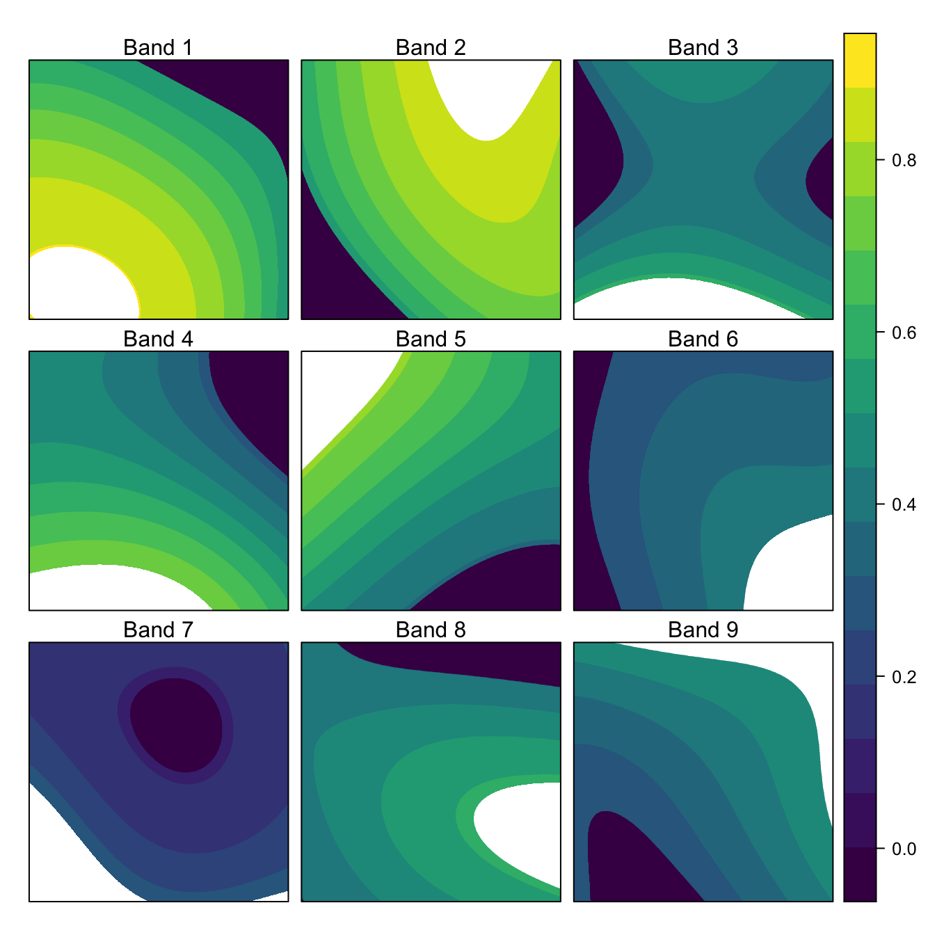
We can calculate the total number of values this raster can store and the associated memory requirements assuming 8 bytes per cell value. To calculate the actual memory used, we can override the default raster behavior and read the contents of the file into R using readAll().
n_values <- ncell(r) * nlayers(r)
# memory in mb
mem_est <- 8 * n_values / 2^20
mem_act <- as.integer(object.size(readAll(r))) / 2^20
#> [1] "# values in raster:  9,000,000"
#> [1] "Estimated size (MB):  68.7"
#> [1] "Memory usage (MB):  68.8"
So we were fairly close in our estimates, looks like it takes a little under 70 Mb of memory to hold this object in the R session.
Processing rasters
Let’s apply the calc() function to this dataset to calculate the cell-wise mean across layers.
r_mean <- calc(r, mean, na.rm = TRUE)This is essentially to equivalent of apply() for a array with 3 dimensions, e.g.:
a <- array(runif(27), dim = c(3, 3, 3))
apply(a, 1:2, mean)
#>       [,1]  [,2]  [,3]
#> [1,] 0.236 0.602 0.570
#> [2,] 0.452 0.412 0.588
#> [3,] 0.561 0.598 0.545
But what raster is doing in calc() is a little different and depends on the memory requirements of the calculation. We can use the function canProccessInMemory() to test whether a Raster* object can be loaded into memory for processing or not. We’ll use verbose = TRUE to get some additional information.
canProcessInMemory(r, verbose = TRUE)
#> memory stats in GB
#> mem available: 5.11
#>         60%  : 3.06
#> mem needed   : 0.27
#> max allowed  : 4.66  (if available)
#> [1] TRUE
This tells me how much free memory I have available on my computer and how much memory is required for this Raster* object. We don’t want raster eating up all our memory, so raster has two user adjustable options to specify the maximum amount of memory it will use in bytes or relative to the available memory. These values default to 5 billion bytes (4.66 GB) and 60%, respectively, but can be adjusted with rasterOptions().
raster functions call canProccessInMemory() when they’re invoked, then use a different approach for processing depending on the results:
canProcessInMemory(r) == TRUE: read the entire object into the R session, then process all at once similar toapply().canProcessInMemory(r) == FALSE: process the raster in blocks of rows, each of which is small enough to store in memory. This approach requires that the output raster object is saved in a file. Blocks of rows are read from the input files, processed in R, then written to the output file, and this is done iteratively for all the blocks until the whole raster is processed.
One wrinkle to this is that each raster function has different memory requirements. This is dealt with using the n argument to canProccessInMemory(), which specifies the number of copies of the Raster* object’s cell values that the function needs to have in memory. Specifically, the estimated memory requirement in bytes is 8 * n * ncell(r) * nlayers(r). Let’s see how different values of n affect whether a raster can be processed in memory:
tibble(n = c(1, 10, 20, 30, 40, 50, 60)) %>%
  mutate(process_in_mem = map_lgl(n, canProcessInMemory, x = r))
#> # A tibble: 7 x 2
#>       n process_in_mem
#>   <dbl> <lgl>
#> 1     1 TRUE
#> 2    10 TRUE
#> 3    20 TRUE
#> 4    30 TRUE
#> 5    40 TRUE
#> 6    50 FALSE
#> 7    60 FALSE
So, even though I called this a “large” raster, R can still handle processing it in memory until we get to requiring a fairly large number of copies, at which time, the raster will switch to being processed in blocks. For reason I don’t fully understand, the source code of the calc() function suggests that it’s using n = 2 * (nlayers(r) + 1), which is 20, so calc() is processing this raster in memory on my system. Indeed, we can confirm that the result of this calculation are stored in a memory with inMemory().
inMemory(r_mean)
#> [1] TRUE
What’s the point of going to all this trouble? If a raster can be processed in blocks to reduce memory usage, why not do it all the time? The issue is that processing in memory is much faster than processing in blocks and having to write to a file. We can see this by forcing calc() to process on disk in blocks by setting rasterOptions(todisk = TRUE).
# in memory
rasterOptions(todisk = FALSE)
t_inmem <- system.time(calc(r, mean, na.rm = TRUE))
print(t_inmem)
#>    user  system elapsed
#>   5.533   0.149   5.699

# on disk
rasterOptions(todisk = TRUE)
t_ondisk <- system.time(calc(r, mean, na.rm = TRUE))
print(t_ondisk)
#>    user  system elapsed
#>   5.683   0.392   6.091
rasterOptions(todisk = FALSE)
So, we see a 6.9% increase in efficiency by processing in memory. The profmem package can gives us some information on the different amounts of memory used for the two approaches. Specifically, we can estimate the maximum amount of memory used at any one time by calc().
# in memory
rasterOptions(todisk = FALSE)
m_inmem <- max(profmem(calc(r, mean, na.rm = TRUE))$bytes, na.rm = TRUE)

# on disk
rasterOptions(todisk = TRUE)
m_ondisk <- max(profmem(calc(r, mean, na.rm = TRUE))$bytes, na.rm = TRUE)
rasterOptions(todisk = FALSE)
#> [1] "In memory (MB):  69"
#> [1] "On disk (MB):  17"
So, it’s clear that different ways of processing Raster* objects affects both the processing time and resource use.
raster options
The raster package has a few options that can adjusted to tweak how functions process data. Let’s take a look at the default values:
rasterOptions()
#> format        : raster
#> datatype      : FLT4S
#> overwrite     : FALSE
#> progress      : none
#> timer         : FALSE
#> chunksize     : 1e+08
#> maxmemory     : 5e+09
#> memfrac       : 0.6
#> tmpdir        : /var/folders/mg/qh40qmqd7376xn8qxd6hm5lwjyy0h2/T//Rtmp3inPgu/raster//
#> tmptime       : 168
#> setfileext    : TRUE
#> tolerance     : 0.1
#> standardnames : TRUE
#> warn depracat.: TRUE
#> header        : none
The options relevant to memory and processing are:
maxmemory: the maximum amount of memory (in bytes) to use for a given operation, defaults to 5 billion bytes (4.66 GB).memfrac: the maximum proportion of the available memory to use for a given operation, defaults to 60%.chunksize: the maximum size (in bytes) of individual chunks of data to read/write when a raster is being processed in blocks, defaults to 100 million bytes (0.1 GB).todisk: used to force processing on disk in blocks.
For example, we can adjust chunksize to force calc() to process our raster stack in smaller pieces. Note that raster actually ignores user specified values of chunksize if they’re below \(10^5\), so I’ll have to do something sketchy and overwrite an internal raster function to allow this.
# hack raster internal function
cs_orig <- raster:::.chunk
cs_hack <- function(x) getOption("rasterChunkSize")
assignInNamespace(".chunk", cs_hack, ns = "raster")

# use 1 kb chunks
rasterOptions(chunksize = 1000, todisk = TRUE)
t_smallchunks <- system.time(calc(r, mean, na.rm = TRUE))

# undo the hack
assignInNamespace(".chunk", cs_orig, ns = "raster")
rasterOptions(default = TRUE)
Processing in smaller chunks resulted in a 56.4% decrease in efficiency compared to the default chunk size. All this suggests to me that, when dealing with large rasters, it makes sense to increase maxmemory as much as feasible given the memory available on your system; the default value of ~ 1 GB is quite small for a modern computer. Then, once you get to a point where the raster has to be processed in blocks, increase chunksize to take advantage of as much memory as you have available.
Processing in blocks
I want to take a quick detour to understand exactly how raster processes data in blocks. Looking at the source code of the calc() function gives a template for how this is done. A few raster functions help with this:
blockSize()suggests a sensible way to break up aRaster*object for processing in blocks. Therasterobjects always uses a set of entire rows as blocks, so this function gives the starting row numbers of each block.readStart()opens a file on disk for reading.getValues()reads a block of data, defined by the starting row and number of rows.readStop()closes the input file.writeStart()opens a file on disk for writing the results of our calculations to.writeValues()writes a block of data to a file, starting at a given row.writeStop()closes the output file.
Let’s set things up to replicate what calc() does. First we need to determine how to dive the input raster up into blocks for processing:
# file paths
f_in <- "data/large-raster.tif"
f_out <- tempfile(fileext = ".tif")

# input and output rasters
r_in <- stack(f_in)
r_out <- raster(r_in)

# blocks
b <- blockSize(r_in)
print(b)
#> $row
#> [1]   1 251 501 751
#>
#> $nrows
#> [1] 250 250 250 250
#>
#> $n
#> [1] 4
So, blockSize() is suggesting we break the file up into 4 blocks (b$n) of 250 (b$nrows) each, and b$rows gives us the starting row value for each block. Now we open the input and output files, process the blocks iteratively, reading and writing as necessary, then close the files.
# open files
r_in <- readStart(r_in)
r_out <- writeStart(r_out, filename = f_out)

# loop over blocks
for (i in seq_along(b$row)) {
  # read values for block
  # format is a matrix with rows the cells values and columns the layers
  v <- getValues(r_in, row = b$row[i], nrows = b$nrows[i])

  # mean cell value across layers
  v <- rowMeans(v, na.rm = TRUE)

  # write to output file
  r_out <- writeValues(r_out, v, b$row[i])
}

# close files
r_out <- writeStop(r_out)
r_in <- readStop(r_in)
That’s it, not particularly complicated! Let’s make sure it worked by comparing to the results from calc().
cellStats(abs(r_mean- r_out), max, na.rm = TRUE)
#> [1] 2.98e-08
Everything looks good, the results are identical! Hopefully, this minimal example is a good template if you want to build your own raster processing functions.
Parallel processing
Breaking a raster up into blocks and processing each independently suggests another approach to more efficient raster processing: parallelization. Each block could be processed by a different core or node and the results will be collected in the output file. Fortunately, raster has some nice tools for parallel raster processing. The function clusterR() essentially takes an existing raster function such as calc() and runs it in parallel. Prior to using it, we need to Here’s how it works:
# start a cluster with four cores
beginCluster(n = 4)
t_parallel <- system.time({
  parallel_mean <- clusterR(r, fun = calc,
                            args = list(fun = mean, na.rm = TRUE))
})
endCluster()

# time for parallel calc
t_parallel[3]
#> elapsed
#>    10.7
# time for sequential calc
t_ondisk[3]
#> elapsed
#>    6.09
Hmmm, there’s something odd going on here, it’s taking longer for the parallel version than the sequential version. I suspect I’ve messed something up in the parallel implementation. Let me know if you know what I’ve done wrong, perhaps it’s a topic for another post.
Matt Strimas-Mackey
Data Scientist
I am a data scientist at the Cornell Lab of Ornithology using data from the citizen science project eBird to inform bird research and conservation.