Lotka-Volterra Predator Prey Model

Last updated on Mar 20, 2020 13 min read

In this post, I’ll explore using R to analyze dynamical systems. Using the Lotka-Volterra predator prey model as a simple case-study, I use the R packages deSolve to solve a system of differential equations and FME to perform a sensitivity analysis.

library(tidyverse)
library(deSolve)
library(FME)

Lotka-Volterra model

The Lotka-Volterra model describes the dynamics of a two-species system in which one is a predator and the other is its prey. The equations governing the dynamics of the prey (with density \(x\) and predator (with density \(y\)) are:

\[ \begin{aligned} \frac{dx}{dt} & = \alpha x - \beta xy \\ \frac{dy}{dt} & = \delta \beta xy - \gamma y \end{aligned} \]

where \(\alpha\) is the (exponential) growth rate of the prey in the absence of predation, \(\beta\) is the predation rate or predator search efficiency, \(\delta\) describes the predator food conversion efficiency, and \(\gamma\) is the predator mortality.

Solving the ODE

Given a set of initial conditions and parameter estimates, deSolve::ode() can be used to evolve a dynamical system described by a set of ODEs. I start by defining parameters, as a named list, and the initial state, as a vector. For the initial state, it is the order that matters not the names.

# parameters
pars <- c(alpha = 1, beta = 0.2, delta = 0.5, gamma = 0.2)
# initial state 
init <- c(x = 1, y = 2)
# times
times <- seq(0, 100, by = 1)

Next, I need to define a function that computes the derivatives in the ODE system at a given point in time.

deriv <- function(t, state, pars) {
  with(as.list(c(state, pars)), {
    d_x <- alpha * x - beta * x * y
    d_y <- delta * beta * x * y - gamma * y
    return(list(c(x = d_x, y = d_y)))
  })
}
lv_results <- ode(init, times, deriv, pars)

The vignette for FME suggets rolling all this into a function as follows. This function will become the input for the FME sensitivity analysis.

lv_model <- function(pars, times = seq(0, 50, by = 1)) {
  # initial state 
  state <- c(x = 1, y = 2)
  # derivative
  deriv <- function(t, state, pars) {
    with(as.list(c(state, pars)), {
      d_x <- alpha * x - beta * x * y
      d_y <- delta * beta * x * y - gamma * y
      return(list(c(x = d_x, y = d_y)))
    })
  }
  # solve
  ode(y = state, times = times, func = deriv, parms = pars)
}
lv_results <- lv_model(pars = pars, times = seq(0, 50, by = 0.25))

The ouput of ode() is a matrix with one column for each state variable. I convert this to a data frame and plot the evolution of the system over time.

lv_results %>% 
  data.frame() %>% 
  gather(var, pop, -time) %>% 
  mutate(var = if_else(var == "x", "Prey", "Predator")) %>% 
  ggplot(aes(x = time, y = pop)) +
    geom_line(aes(color = var)) +
    scale_color_brewer(NULL, palette = "Set1") +
    labs(title = "Lotka-Volterra predator prey model",
         subtitle = paste(names(pars), pars, sep = " = ", collapse = "; "),
         x = "Time", y = "Population density")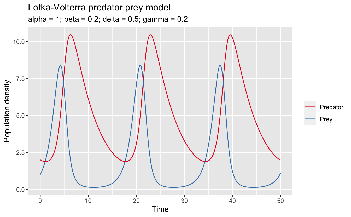

This choice of paramters leads to periodic dynamics in which the prey population initially increases, leading to an abundance of food for the predators. The predators increase in response (lagging the prey population), eventually overwhelming the prey population, which crashes. This in turn causes the predators to crash, and the cycle repeats. The period of these dynamics is about 15 seconds, with the predators lagging the prey by about a second.

Sensitivity analysis

A sensitivity analysis examines how changes in the parameters underlying a model affect the behaviour of the system. It can help us understand the impact of uncertainty in parameter estimates. The FME vignette covers two types of sensitivity analyses: global and local.

Global sensitivity

According to the FME vingette, in a global sensitivity analysis certain parameters (the sensitivity parameters) are varied over a large range, and the effect on model output variables (the sensitivity variables) is measured. To accomplish this, a distribution is defined for each sensitivity parameter and the model is run multiple times, each time drawing values for the sensistivity parameters from their distribution. The sensitivity variables are recorded for each iteration over a range of times. The function sensRange() carries out global sensitivity analyses.

I’ll look at the sensitivity of the populations to the growth rate (\(\alpha\)) and the predation rate (\(\beta\)). Defining the sensitivity parameter distributions requires providing a data frame in which the first column is the minimum value, the second column the maximum, and the row names are the parameter names.

par_ranges <- data.frame(min = c(0.75, 0.15),
                         max = c(1.25, 0.25),
                         row.names = c("alpha", "beta"))
par_ranges
#>        min  max
#> alpha 0.75 1.25
#> beta  0.15 0.25

Now I use sensRange() to solve the models over the range of parameters. The argument dist = "grid" sets the sensitivity parameter distribution to a regular grid of values, sensvar defines which variables are the sensitivity variables (i.e. the ones whose time series will be returned in the output), num is the number of iterations and therefore the number of different sensistivity parameter values (note that if there are \(k\) sensitivity parameters, num must have an integer \(k\)th root), and times is the time series over which to evaluate the model.

The output of this function is a data frame with rows corresponding to the different sensitivity parameter values and columns corresponding to the combination of time steps and sensitivity variables. So, for n time steps, there are n columns for each sensitivity variable. First I run a simple sensitivity analysis to aid examination of the output.

lv_glob_sens <- sensRange(func = lv_model, parms = pars, dist = "grid",
                          sensvar = c("x", "y"), parRange = par_ranges,
                          num = 4, times = seq(0, 1, by = 0.5))
lv_glob_sens
#>   alpha beta x0 x0.5   x1 y0 y0.5   y1
#> 1  0.75 0.15  1 1.26 1.59  2 1.89 1.80
#> 2  1.25 0.15  1 1.61 2.62  2 1.90 1.86
#> 3  0.75 0.25  1 1.14 1.30  2 1.93 1.89
#> 4  1.25 0.25  1 1.46 2.14  2 1.95 1.97

Here variables such as x0.5 refer to the values of \(x\) at \(t=0.5\). FME provides a plot() method for sensRange objects, which adds envelopes to the variables showing the range and mean ± standard deviation. Now I run a more realistic sensitivity analysis and produce the plots. Note that summary() must be called before plot() to get the desired plots.

lv_glob_sens <- sensRange(func = lv_model, parms = pars, dist = "grid",
                          sensvar = c("x", "y"), parRange = par_ranges,
                          num = 100, times = seq(0, 50, by = 0.25))
lv_glob_sens %>% 
  summary() %>% 
  plot(main = c("Prey", "Predator"),
       xlab = "Time", ylab = "Population density",
       col = c("lightblue", "darkblue"))
mtext("Sensitivity to alpha and beta", outer = TRUE, line = -1.5, side = 3, 
      cex = 1.25)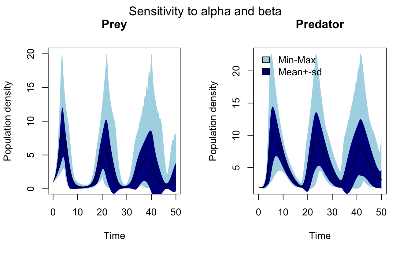

To actually work with these data, I’ll transform the data frame from wide to long format using tidyr. gather() converts from wide to long format, then separate() splits column names x1.5 into two fields: one identifying the variable (x) and one specifying the time step (1.5).

lv_sens_long <- lv_glob_sens %>% 
  gather(key, abundance, -alpha, -beta) %>% 
  separate(key, into = c("species", "t"), sep = 1) %>% 
  mutate(t = parse_number(t)) %>% 
  select(species, t, alpha, beta, abundance)
head(lv_sens_long)
#>   species t alpha beta abundance
#> 1       x 0 0.750 0.15         1
#> 2       x 0 0.806 0.15         1
#> 3       x 0 0.861 0.15         1
#> 4       x 0 0.917 0.15         1
#> 5       x 0 0.972 0.15         1
#> 6       x 0 1.028 0.15         1
glimpse(lv_sens_long)
#> Observations: 40,200
#> Variables: 5
#> $ species   <chr> "x", "x", "x", "x", "x", "x", "x", "x", "x", "x", "x", "x",…
#> $ t         <dbl> 0, 0, 0, 0, 0, 0, 0, 0, 0, 0, 0, 0, 0, 0, 0, 0, 0, 0, 0, 0,…
#> $ alpha     <dbl> 0.750, 0.806, 0.861, 0.917, 0.972, 1.028, 1.083, 1.139, 1.1…
#> $ beta      <dbl> 0.150, 0.150, 0.150, 0.150, 0.150, 0.150, 0.150, 0.150, 0.1…
#> $ abundance <dbl> 1, 1, 1, 1, 1, 1, 1, 1, 1, 1, 1, 1, 1, 1, 1, 1, 1, 1, 1, 1,…

Now, I can, for example, recreate the above plot with ggplot2. First, I summarize the data to calculate the envelopes, then I plot.

lv_sens_summ <- lv_sens_long %>% 
  group_by(species, t) %>% 
  summarize(a_mean = mean(abundance),
            a_min = min(abundance), a_max = max(abundance),
            a_sd = sd(abundance)) %>% 
  ungroup() %>% 
  mutate(a_psd = a_mean + a_sd, a_msd = a_mean - a_sd,
         species = if_else(species == "x", "Prey", "Predator"),
         species = factor(species, levels = c("Prey", "Predator")))
ggplot(lv_sens_summ, aes(x = t, group = species)) +
  # mean+-sd
  geom_ribbon(aes(ymin = a_msd, ymax = a_psd, fill = species), alpha = 0.2) +
  # mean
  geom_line(aes(y = a_mean, color = species)) +
  labs(title = "Sensitivity to alpha and beta (mean ± sd)", 
       subtitle = "alpha = [0.75, 1.25]; beta = [0.15, 0.25]",
       x = "Time", y = "Population density") +
  scale_color_brewer(NULL, palette = "Set1") +
  scale_fill_brewer(NULL, palette = "Set1")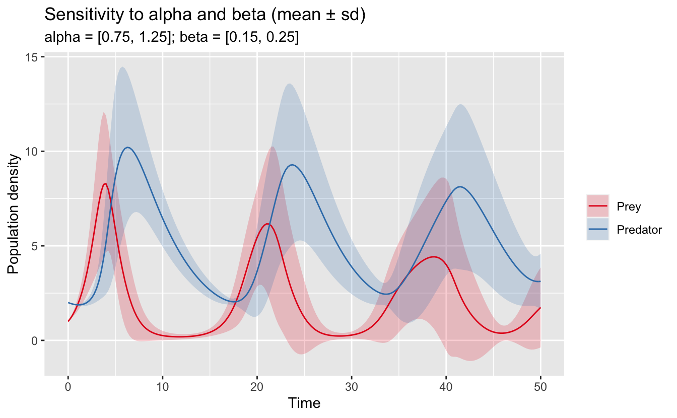

In this format, it’s also easy to fix one of the values for a sensitivity parameter and only vary the other one.

lv_sens_summ <- lv_sens_long %>% 
  # fix beta at 0.15
  filter(beta == 0.15) %>% 
  group_by(species, t) %>% 
  summarize(a_mean = mean(abundance),
            a_min = min(abundance), a_max = max(abundance),
            a_sd = sd(abundance)) %>% 
  ungroup() %>% 
  mutate(a_psd = a_mean + a_sd, a_msd = a_mean - a_sd,
         species = if_else(species == "x", "Prey", "Predator"),
         species = factor(species, levels = c("Prey", "Predator")))
ggplot(lv_sens_summ, aes(x = t, group = species)) +
  # mean+-sd
  geom_ribbon(aes(ymin = a_msd, ymax = a_psd, fill = species), alpha = 0.2) +
  # mean
  geom_line(aes(y = a_mean, color = species)) +
  labs(title = "Sensitivity to alpha at fixed beta (mean ± sd)", 
       subtitle = "alpha = [0.75, 1.25]; beta = 0.15",
       x = "Time", y = "Population density") +
  scale_color_brewer(NULL, palette = "Set1") +
  scale_fill_brewer(NULL, palette = "Set1")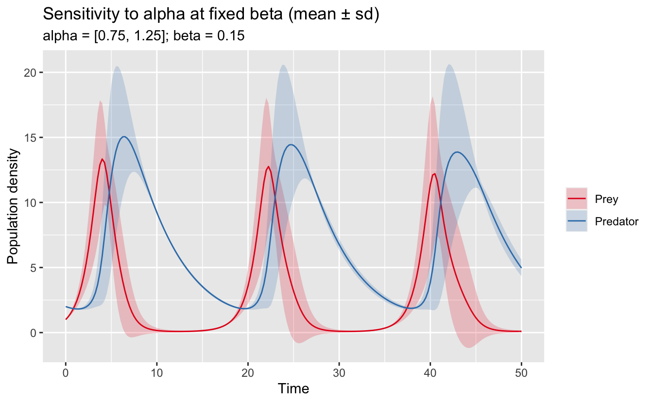

Local sensitivity analysis

According to the FME vingette, in a local sensitivity analysis, “the effect of a parameter value in a very small region near its nominal value is estimated”. The method used by FME is to calculate a matrix of sensitivity functions, \(S_{i,j}\), defined by:

\[ S_{i,j} = f(v_i, p_i) = \frac{dv_i}{dp_j} \frac{s_{p_j}}{s_{v_i}} \]

where \(v_i\) is a sensitivity variable \(i\) (which is dependent on time \(t\)), \(p_j\) is sensitivity parameter \(j\), and \(s_{v_i}\) and \(s_{p_j}\) are scaling factors for variables and parameters, respectively. By default, FME takes the scaling values to be equal to the underlying quantities, in which case the above equation simplifies to:

\[ S_{i,j} = f(v_i, p_i) = \frac{dv_i}{dp_j} \frac{p_j}{v_i} \]

The function sensFun() is used to numerically estimate these sensitivity functions at a series of time steps. The arguments sensvar and senspar are used to define which variables and parameters, respectively, will be investigated in the sensitivity analysis. By default, all variables are parameters are included. The arguments varscale and parscale define the scaling factors; however, for now, I’ll leave them blank, which sets them to the underlying quantities as in the above equation.

In practice, sensFun() works by applying a small perturbation, \(\delta_j\), to parameter \(j\), solving the model for a range of time steps to determine \(v_i\), then taking the ratio of the changes to the parameters and variables. The perturbation is defined by the argument tiny as \(\delta_j = \text{max}(tiny, tiny * p_j)\). tiny defaults to \(10^{-8}\).

To test that sensFun() is doing what I think it is, I’ll implement a version of it. For simplicity, I’ll only consider the variable \(x\) (prey density):

sen_fun <- function(fun, pars, times, tiny = 1e-8) {
  # the unperturbed values, just x
  v_unpert <- fun(pars, times)[, "x"]
  # loop over parameters, pertuburbing each in turn
  s_ij <- matrix(NA, nrow = length(times), ncol = (1 + length(pars)))
  s_ij[, 1] <- times
  colnames(s_ij) <- c("t", names(pars))
  for (j in seq_along(pars)) {
    # perturb the ith parameter
    delta <- max(tiny, abs(tiny * pars[j]))
    p_pert <- pars
    p_pert[j] <- p_pert[j] + delta
    # solve model
    v_pert <- fun(pars = p_pert, times = times)[, "x"]
    # calculate the resulting difference in variables at each timestep, just x
    delta_v <- (v_pert - v_unpert)
    # finally, calculate the sensitivity function at each time step
    s_ij[, j + 1] <- (delta_v / delta) * (pars[j] / v_unpert)
  }
  return(s_ij)
}

Now I compare this implementation to the actual results.

test_pars <- c(alpha = 1.5, beta = 0.2, delta = 0.5, gamma = 0.2)
sen_fun(lv_model, pars = test_pars, times = 0:2)
#>      t alpha   beta  delta  gamma
#> [1,] 0  0.00  0.000  0.000 0.0000
#> [2,] 1  1.48 -0.415 -0.029 0.0386
#> [3,] 2  2.69 -0.966 -0.210 0.1655
sensFun(lv_model, parms = test_pars, sensvar = "x", times = 0:2)
#>   x var alpha   beta  delta  gamma
#> 1 0   x  0.00  0.000  0.000 0.0000
#> 2 1   x  1.48 -0.415 -0.029 0.0386
#> 3 2   x  2.69 -0.966 -0.210 0.1655

A perfect match! Now that I know what sensFun() is actually doing, I’ll put it to use to solve the original LV model. One difference here is that I’ll consider both variables as sensitivity variables and the results for each variable will be stacked rowwise. In addition, in the FME documentation, \(s_{v_i}\) is set to 1, which is on the order of the actual variable values, but has the benefit of being constant over time. I’ll do the same here.

lv_loc_sens <- sensFun(lv_model, parms = pars, varscale = 1, 
                       times = seq(0, 50, by = 0.25))
head(lv_loc_sens)
#>      x var alpha   beta    delta   gamma
#> 1 0.00   x 0.000  0.000  0.00000 0.00000
#> 2 0.25   x 0.291 -0.116 -0.00151 0.00286
#> 3 0.50   x 0.677 -0.272 -0.00729 0.01316
#> 4 0.75   x 1.182 -0.478 -0.01997 0.03413
#> 5 1.00   x 1.833 -0.749 -0.04341 0.07015
#> 6 1.25   x 2.663 -1.104 -0.08330 0.12706
tail(lv_loc_sens)
#>        x var alpha  beta  delta gamma
#> 397 48.8   y -1.95 -5.45 -0.933 -9.07
#> 398 49.0   y -1.81 -4.95 -0.831 -8.38
#> 399 49.2   y -1.66 -4.43 -0.725 -7.64
#> 400 49.5   y -1.49 -3.90 -0.614 -6.87
#> 401 49.8   y -1.30 -3.34 -0.495 -6.04
#> 402 50.0   y -1.08 -2.75 -0.367 -5.15

summary() can be used to summarize these results over the time series, for example, to see which parameters the model is most sensitive too.

summary(lv_loc_sens)
#>       value scale   L1   L2 Mean Min Max   N
#> alpha   1.0   1.0  6.5 11.2  2.2 -35  44 402
#> beta    0.2   0.2  8.3 12.5 -4.1 -56  33 402
#> delta   0.5   0.5  2.5  4.3 -1.1 -19  11 402
#> gamma   0.2   0.2 10.8 18.2 -0.1 -78  74 402

\(\gamma\) (predator mortality rate) and \(\beta\) (predator search efficiency) have the largest values for the sensitivity function, on average, suggesting that this model is most sensitive to these parameters. There is also plot method for the output of sensFun(), which plots the sensitivity functions as time series.

plot(lv_loc_sens)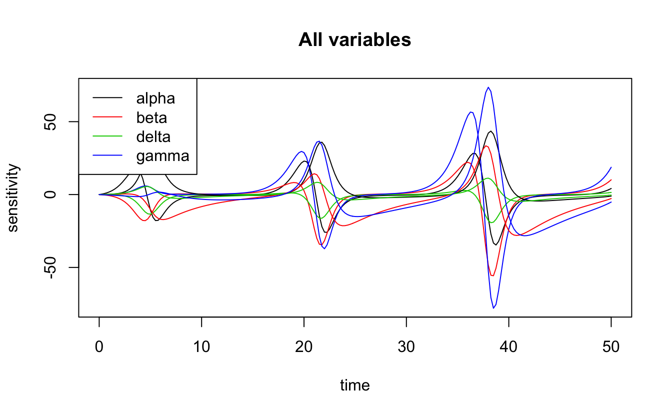

However, it’s also possible to use ggplot2 provided I transpose the data to long format first.

lv_loc_long <- lv_loc_sens %>% 
  gather(parameter, sensitivity, -x, -var) %>% 
  mutate(var = if_else(var == "x", "Prey", "Predator"))
ggplot(lv_loc_long, aes(x = x, y = sensitivity)) +
  geom_line(aes(colour = parameter, linetype = var)) +
  scale_color_brewer("Parameter", palette = "Set1") +
  scale_linetype_discrete("Variable") +
  labs(title = "Lotka-Volterra parameter sensitivity functions", 
       subtitle = paste(names(pars), pars, sep = " = ", collapse = "; "),
       x = "Time", y = "Sensitivity") + 
  theme(legend.position = "bottom")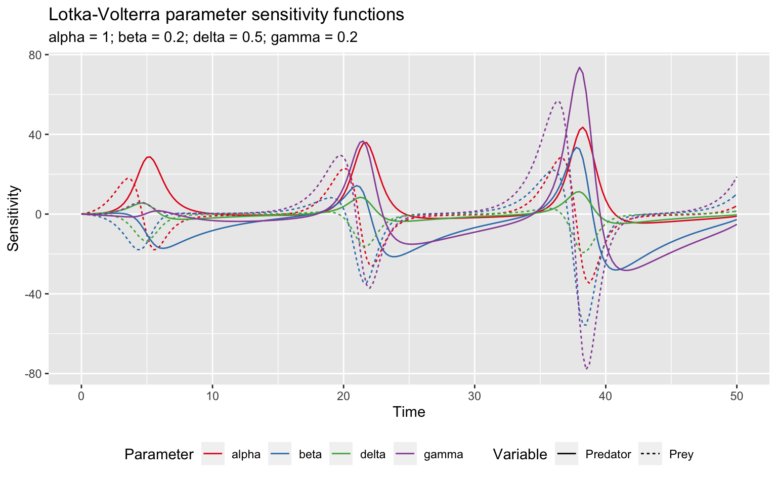

Clearly this model is particularly sensitive to \(\gamma\). Furthermore, this sensitivity shows peaks every 16 seconds or so, which is the periodicity of the original dynamics. To see what’s going on here, I’ll take a look at what happens to the two species when I increase \(\gamma\) by 1%:

# original model
lv_results <- lv_model(pars, times = seq(0, 50, by = 0.25)) %>% 
  data.frame() %>% 
  gather(var, pop, -time) %>% 
  mutate(var = if_else(var == "x", "Prey", "Predator"),
         par = as.character(pars["gamma"]))
# perturbed model
new_pars <- pars
new_pars["gamma"] <- new_pars["gamma"] * 1.1
lv_results_gamma <- lv_model(new_pars, times = seq(0, 50, by = 0.25)) %>% 
  data.frame() %>% 
  gather(var, pop, -time) %>% 
  mutate(var = if_else(var == "x", "Prey", "Predator"),
         par = as.character(new_pars["gamma"]))
# plot
ggplot(bind_rows(lv_results, lv_results_gamma), aes(x = time, y = pop)) +
  geom_line(aes(color = var, linetype = par)) +
  scale_color_brewer("Species", palette = "Set1") +
  scale_linetype_discrete("gamma") +
  labs(title = "Lotka-Volterra predator prey model",
       subtitle = "Increasing gamma leads to period increasing with time",
       x = "Time", y = "Population density") +
  theme(legend.position = "bottom")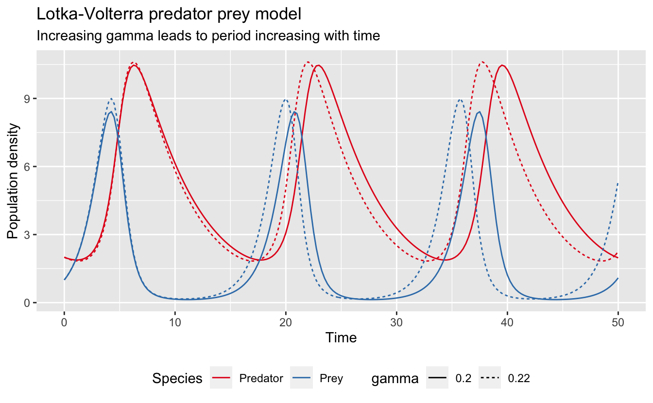

Increasing \(\gamma\) leads to a time dependent period to the dynamics. As a result, the two models initially overlap, but they become increasingly out of sync over time. This explains both the periodicity of the sensitivity function and the increasing amplitude.

R Ecology

Matt Strimas-Mackey

Data Scientist

I am a data scientist at the Cornell Lab of Ornithology using data from the citizen science project eBird to inform bird research and conservation.