Efficient Block Processing of Rasters in R

Modifying the raster package

After forking the raster package repository I made the following changes:

1. calc() now displays the block size (i.e. number of rows) being used.
2. calc(return_blocks = TRUE) will, instead of processing the raster object, just return the blocks that would have been used.
3. Added a new function, summarize_raster(), that’s a simplified version of calc(). It always process files on disk, will only calculate means and sums rather than a generic input function, always uses na.rm = TRUE, and it takes either a chunksize argument (in units of available GB of RAM) or an n_rows argument that directly controls the number of rows per block.

If you’re interested, the source code for the summarize_raster() function is here. It removes much of the functionality of calc() but this comes with the benefit of being easier to figure out what’s going on inside the function. If you want to install this version of the raster package you could do so with remotes::install_github("mstrimas/raster"), but beware I’ve modified the original package in a very sloppy way and you probably don’t want to overwrite the real raster package with my hacked version.

So, what block size is being used?

tic()
r_mean_calc <- calc(r, mean, na.rm = TRUE)
#> Using 111 blocks of 51 rows.
toc()
#> 127.619 sec elapsed

In this case, with the default chunk size of \(10^8 \approx 0.1 GB\), calc() processes this raster in 111 blocks of 51 rows each. We can use my custom summarize_raster() function to do the same thing, but specify block size explicitly.

tic()
r_mean_summ <- summarize_raster(r, "mean", n_rows = 51)
#> Using 111 blocks of 51 rows.
toc()
#> 125.852 sec elapsed

Turns out summarize_raster() is slightly faster because I’ve slimmed it down and removed some additional checks and functionality. We can confirm that the two approaches produce the same results.

cellStats(abs(r_mean_calc - r_mean_summ), max)
#> [1] 0

Run time vs. block size

Ok, now everything’s in place, and we can examine how block size impacts processing time. Recall that block size is the number of rows that get read in, summarized, and output at each iteration of the processing. Let’s estimate run time for a range of blocks sizes, from 1 row to 5,630 rows, equivalent to processing the whole raster in memory. Note that I’m running this on my laptop, which has 16 GB of RAM, so I have more than enough resources to process this raster in memory, but I’m choosing to process it on disk for demonstration purposes. Since there could be variation in run time, I’ll summarize the raster 10 times for each block size.

# choose the values of n_rows to try
n_rows <- 2^seq(0, ceiling(log2(nrow(r))))
n_rows[length(n_rows)] <- nrow(r)

# set up 10 repetitions of each n_rows value
nrow_grid <- expand_grid(rep = 1:10, n_rows = n_rows)

# summarize raster using each value of n_rows
summarize_nrows <- function(x) {
  # memory usage
  m <- profmem({
    # timer
    t <- system.time({
      r_mean <- summarize_raster(r, "mean", n_rows = x)
    })
  })
  return(tibble(elapsed = t["elapsed"], max_mem = max(m$bytes, na.rm = TRUE)))
}
time_mem <- nrow_grid %>% 
  mutate(results = map(n_rows, summarize_nrows)) %>% 
  unnest(cols = results)

Now let’s plot the elapsed time vs. block size curve. I’ll show both the raw data, consisting of 10 for each block size, and a smoothed function.

ggplot(time_mem) +
  aes(x = n_rows, y = elapsed / 60) +
  geom_point(alpha = 0.25, size = 0.75) +
  geom_smooth(method = "gam") +
  labs(x = "# of rows/block size (log2 scale)", 
       y = "Elapsed time (minutes)")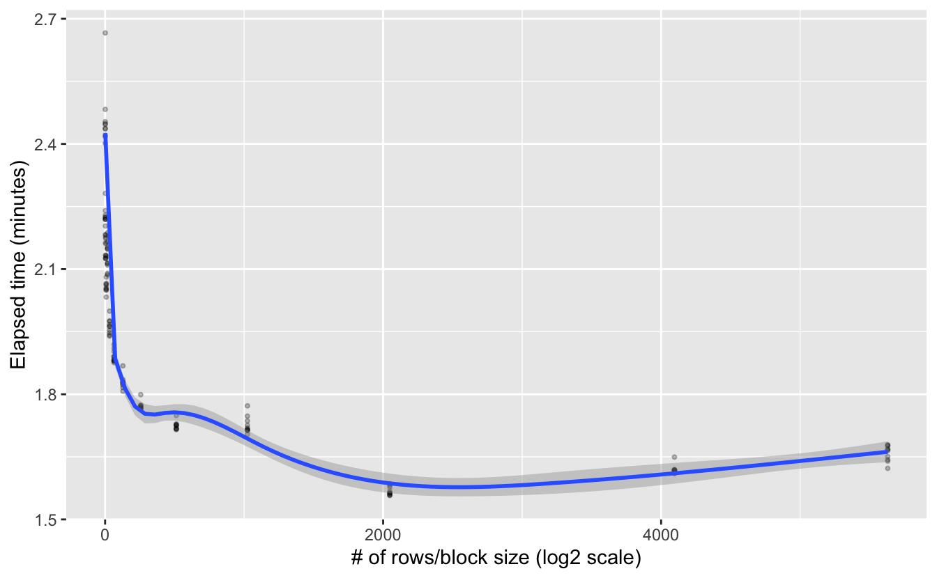

Interesting, it looks like there’s an exponential decrease in processing time as block size increases. This suggests a log-transformed x-axis would be worthwhile. I’m also going to show the default block size explicitly on the plot.

ggplot(time_mem) +
  aes(x = n_rows, y = elapsed / 60) +
  geom_point(alpha = 0.25, size = 0.75) +
  geom_smooth(method = "gam") +
  geom_vline(xintercept = 51,
             color = "orange",
             size = 1.2,
             linetype = "dashed") +
  scale_x_continuous(trans = "log2") +
  labs(x = "# of rows/block size (log2 scale)", 
       y = "Elapsed time (minutes)",
       title = "Processing time decreases exponentially with block size",
       subtitle = "Default block size (51 rows) shown in oranges")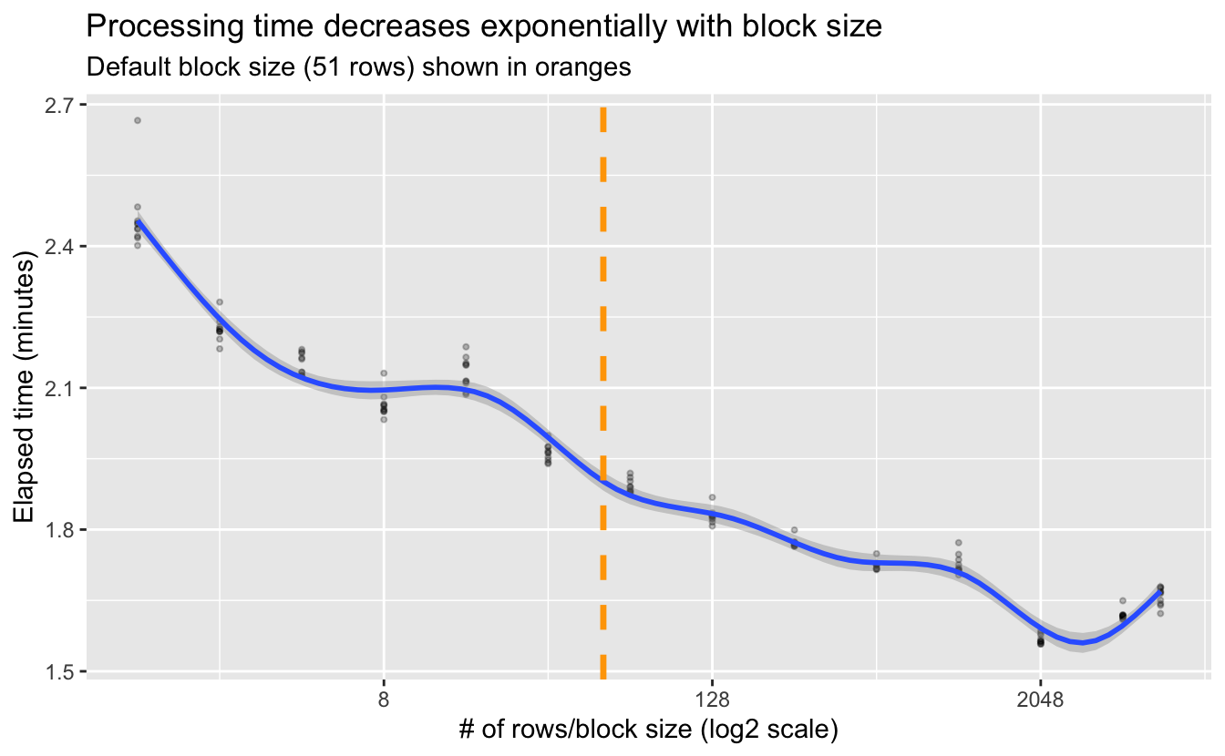

Looks like the decrease is exponential. The default block size using chunksize = 1e8 does a pretty good job, but it’s not giving us the most efficient processing given the memory resources available. This shouldn’t be too surprising since \(10^8\) bytes is quite small, so would should really be picking something more appropriate for our system’s available RAM. All this said, it’s worth noting these are fairly modest efficiency gains, but they can add up if you’re dealing with a large number of big raster files.

I also estimated the maximum memory usage during the summarization, so let’s take a look at that.

ggplot(time_mem) +
  aes(x = n_rows, y = max_mem / 2^30) +
  geom_line() +
  geom_point() +
  labs(x = "# of rows", y = "Maximum memory used (GB)",
       title = "Memory usage increases linearly with block size")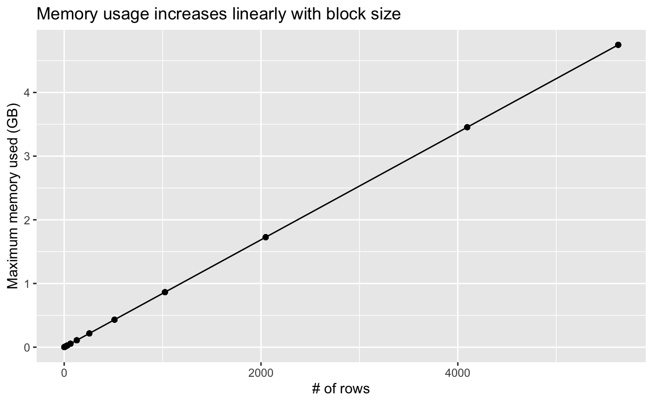

This is as expected: large blocks mean more data is being processed at once, which leads to higher memory usage.

The takeaway from all this is so obvious it’s almost embarrassing: if you want to process large rasters efficiently, increase the chunksize option so the raster package will process files in larger blocks and take advantage of the RAM you have available. Despite it being obvious, I suspect most people are like me and blindly go with the default raster options, which is fine in many cases, but becomes problematic for large rasters.