Raster Summarization in Python

gdal_summarize.py

The goal of gdal-summarize.py is to summarize raster data across layers or bands. There are two common use cases for this tool. The first is calculating a cell-wise summary across the bands of a raster file (e.g. a GeoTIFF). For example, given a multi-band input GeoTIFF file input.tif, to calculate the cell-wise sum of the first three bands use:

gdal-summarize.py input.tif --bands 1 2 3 --outfile output.tif

Alternatively, to compute the cell-wise sum across multiple GeoTIFF files (input1.tif, input2.tif, and input3.tif) use:

gdal-summarize.py input1.tif input2.tif input3.tif --outfile output.tif

If these input files have multiple bands, the default behavior is to summarize them across the first band of each file; however, the --bands argument can override this behavior:

# summarize across the second band of each file
gdal-summarize.py input1.tif input2.tif input3.tif --bands 2 --outfile output.tif
# summarize across band 1 of input1.tif and band 2 of input2.tif
gdal-summarize.py input1.tif input2.tif --bands 1 2 --outfile output.tif

Comparing Python and R

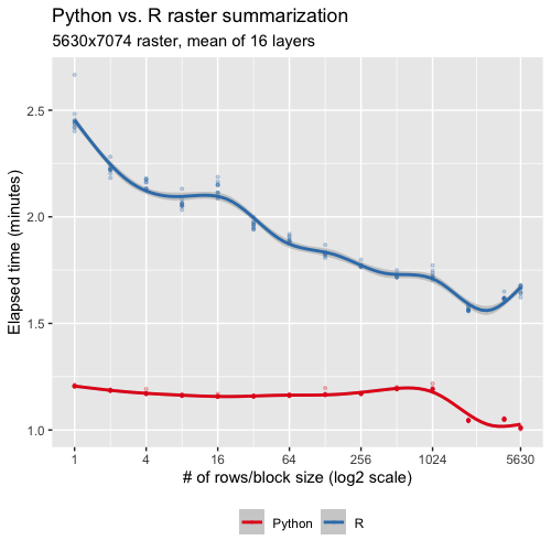
Everyone loves a good Python vs. R battle, so let’s put calc() from the raster R package up against gdal-summarize.py. I use the same Wood Thrush relative abundance raster from eBird Status and Trends as I used in my previous post, consisting of 16 bands with dimensions 5630X7074. Since raster processes data in blocks of rows, I’ll do the same thing for gdal-summarize.py.

library(raster)
library(tidyverse)

f <- "data/woothr.tif"
r <- stack(f)

# choose the values of n_rows to try
n_rows <- 2^seq(0, ceiling(log2(nrow(r))))
n_rows[length(n_rows)] <- nrow(r)

# set up 10 repetitions of each n_rows value
nrow_grid <- expand_grid(rep = 1:10, n_rows = n_rows)

# summarize raster using each value of n_rows
summarize_nrows <- function(x) {
  # time r
  t_r <- system.time({
    r_mean <- summarize_raster(r, "mean", n_rows = x)
  })
  # time python
  f_out <- "woothr-mean.tif"
  t_py <- system.time({
    str_glue("source ~/.bash_profile;",
             "gdal-summarize.py {f} -o {f_out} -w -f 'mean' -n {x}") %>% 
      system()
  })
  tibble(elapsed_r = t_r["elapsed"], elapsed_py = t_py["elapsed"])
}
time_summarize <- nrow_grid %>% 
  mutate(results = map(n_rows, summarize_nrows)) %>% 
  unnest(cols = results)

Let’s take look at how they compare:

# x-axis breaks
brks <- 2^seq(0, ceiling(log2(nrow(r))), by = 2)
brks[length(brks)] <- nrow(r)

# transform to longer for ggplot
time_summarize <- time_summarize %>% 
  pivot_longer(cols = c(elapsed_r, elapsed_py)) %>% 
  mutate(name = recode(name, "elapsed_r" = "R", "elapsed_py" = "Python"))

# plot
ggplot(time_summarize) +
  aes(x = n_rows, y = value / 60, group = name, color = name) +
  geom_point(alpha = 0.25, size = 0.75) +
  geom_smooth(method = "gam") +
  scale_x_continuous(trans = "log2", breaks = brks) +
  scale_color_brewer(palette = "Set1") +
  labs(x = "# of rows/block size (log2 scale)", 
       y = "Elapsed time (minutes)",
       color = NULL,
       title = "Python vs. R raster summarization",
       subtitle = "5630x7074 raster, mean of 16 layers") +
  theme(legend.position = "bottom")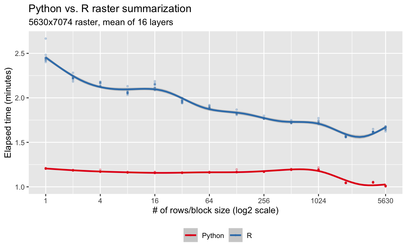

So, not only is Python raster than R, but Python experiences much less of a block size effect.

Hopefully others will find this tool useful! Please take a look through the GitHub repo and let me know if there’s something I could be doing differently. As I said at the start, this is my first foray into Python, so I’m bound to have made some mistakes.