Make an HCL palette for visualizing a linear sequence of distributions
Source:R/palette.R
palette_timeline.RdThis function generates an HCL palette for visualizing a linear sequence of distributions (e.g., a series of utilization distributions describing space use by an individual animal across each of 20 consecutive days or a series of species distributions describing projected responses to global warming in 0.5 C increments).
palette_timeline(x, start_hue = -130, clockwise = FALSE)Arguments
- x
RasterStack or integer describing the number of layers for which colors need to be generated.
- start_hue
integer between -360 and 360 representing the starting hue in the color wheel. For further details, consult the documentation for colorspace::rainbow_hcl. Recommended values are -130 ("blue-pink-yellow" palette) and 50 ("yellow-green-blue" palette).
- clockwise
logical indicating which direction to move around an HCL color wheel. When
clockwise = FALSEthe ending hue will bestart_hue + 180. Whenclockwise = TRUEthe ending hue will bestart_hue - 180. The default valueclockwise = FALSEwill yield a "blue-pink-yellow" palette whenstart_hue = -130, whileclockwise = TRUEwill yield a "blue-green-yellow" palette.
Value
A data frame with three columns:
layer_id: integer identifying the layer containing the maximum intensity value; mapped to hue.specificity: the degree to which intensity values are unevenly distributed across layers; mapped to chroma.color: the hexadecimal color associated with the given layer and specificity values.
See also
palette_timecycle for cyclical sequences of distributions and palette_set for unordered sets of distributions.
Other palette:
palette_set(),
palette_timecycle()
Examples
# load fisher data
data(fisher_ud)
# generate hcl color palette
pal_a <- palette_timeline(fisher_ud)
head(pal_a)
#> specificity layer_id color
#> 1 0 1 #6A6A6A
#> 2 0 2 #6A6A6A
#> 3 0 3 #6A6A6A
#> 4 0 4 #6A6A6A
#> 5 0 5 #6A6A6A
#> 6 0 6 #6A6A6A
# use a clockwise palette
pal_b <- palette_timeline(fisher_ud, clockwise = TRUE)
# try a different starting hue
pal_c <- palette_timeline(fisher_ud, start = 50)
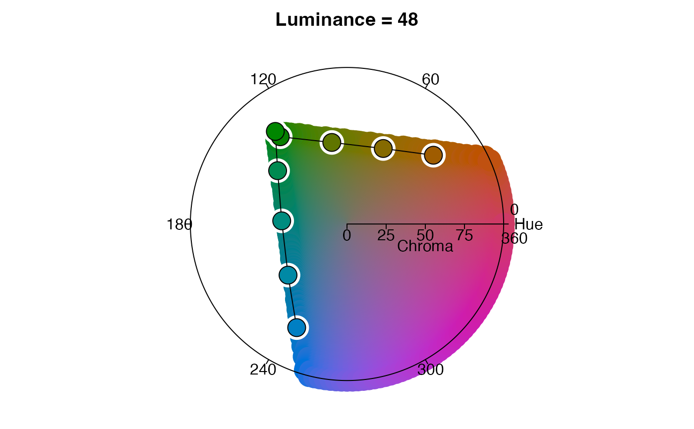
# visualize the palette in HCL space with colorspace::hclplot
library(colorspace)
hclplot(pal_a[pal_a$specificity == 100, ]$color)
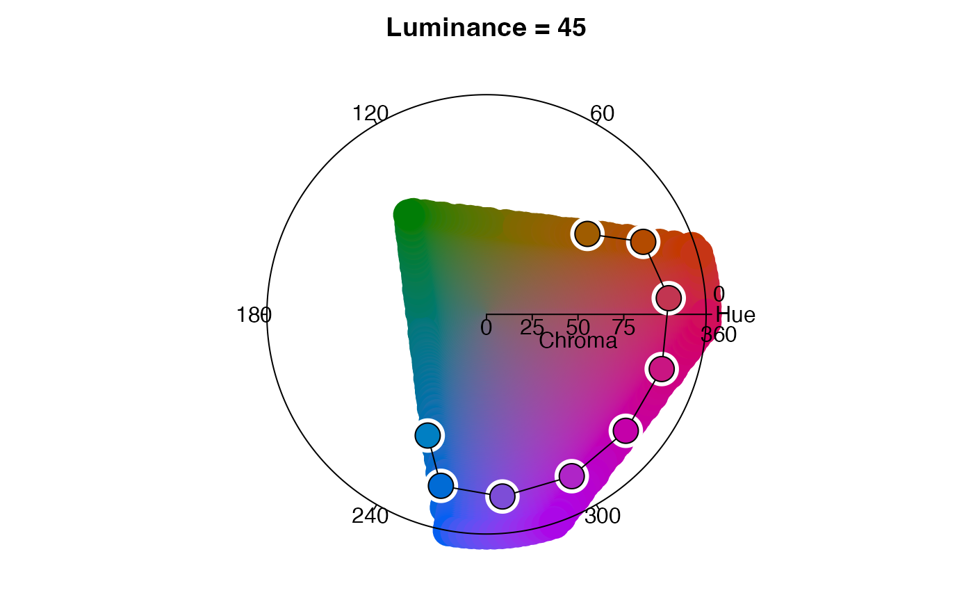 hclplot(pal_b[pal_b$specificity == 100, ]$color)
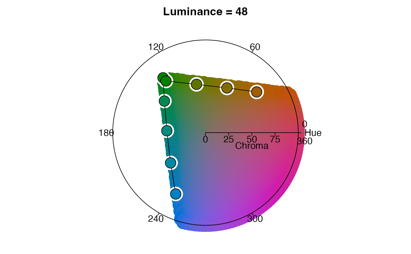 hclplot(pal_c[pal_c$specificity == 100, ]$color)