This function enables visualization of distributional information in a series of small multiples by combining distribution metrics and an HCL color palette.
map_multiples(
  x,
  palette,
  ncol,
  lambda_i = 0,
  labels = NULL,
  return_type = c("plot", "df")
)
Arguments
- x
RasterStack of distributions processed by
metrics_pull().- palette
data frame containing an HCL color palette generated using
palette_timecycle(),palette_timeline(), orpalette_set().- ncol
integer specifying the number of columns in the grid of plots.
- lambda_i
number that allows visual tuning of intensity values via the
scales::modulus_trans()function (see Details). Negative numbers increase the opacity of cells with low intensity values. Positive numbers decrease the opacity of cells with low intensity values.- labels
character vector of layer labels for each plot. The default is to not show labels.
- return_type
character specifying whether the function should return a
ggplot2plot object ("plot") or data frame ("df"). The default is to return aggplot2object.
Value
By default, or when return_type = "plot", the function returns a
map that is a ggplot2 plot object.
When return_type = "df", the function returns a data frame containing
eight columns:
x,y: coordinates of raster cell centers.cell_number: integer indicating the cell number.layer_cell: a unique ID for the cell within the layer in the format"layer-cell_number".intensity: maximum cell value across layers divided by the maximum value across all layers and cells; mapped to alpha level.specificity: the degree to which intensity values are unevenly distributed across layers; mapped to chroma.layer_id: the identity of the raster layer from which an intensity value was pulled; mapped to hue.color: the hexadecimal color associated with the given layer and specificity values.
Details
The lambda_i parameter allows for visual tuning of intensity
values with unusual distributions. For example, distributions often
contain highly skewed intensity values because individuals spend a vast
majority of their time within a relatively small area or because
populations are relatively dense during some seasons and relatively
dispersed during others. This can make visualizing distributions a
challenge. The lambda_i parameter transforms intensity values via the
scales::modulus_trans() function, allowing users to adjust the relative
visual weight of high and low intensity values.
See also
Other map:
map_single()
Examples
# load fisher data
data("fisher_ud")
# prepare data
r <- metrics_pull(fisher_ud)
# generate palette
pal <- palette_timeline(fisher_ud)
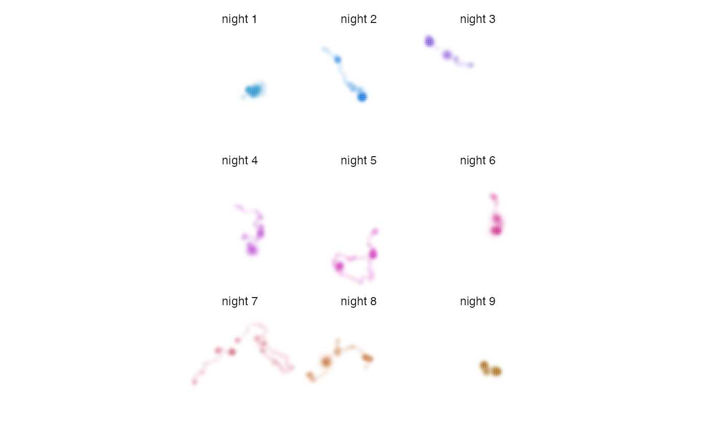
# produce maps, adjusting lambda_i to make areas that were used less
# intensively more conspicuous
map_multiples(r, pal, lambda_i = -5, labels = paste("night", 1:9))