Visualize distributions in a single map

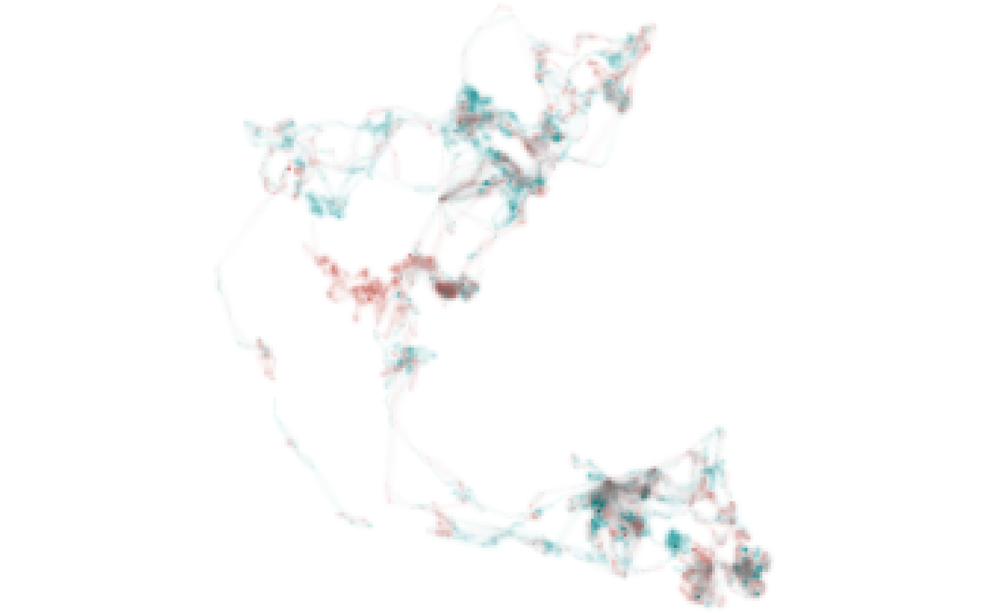
This function enables visualization of distributional information in a single map by combining distribution metrics and an HCL color palette.

map_single(
  x,
  palette,
  layer,
  lambda_i = 0,
  lambda_s = 0,
  return_type = c("plot", "stack", "df")
)

Arguments

x	RasterStack of distributions processed by metrics_pull() or metrics_distill().
palette	data frame containing an HCL color palette generated using palette_timecycle(), palette_timeline(), or palette_set().
layer	integer (or character) corresponding to the layer ID (or name) of layer. A single distribution from within x is mapped when the layer argument is specified. The layer argument is ignored if metrics_distill() was used to generate x.
lambda_i	number that allows visual tuning of intensity values via the scales::modulus_trans() function (see Details). Negative numbers increase the opacity of cells with low intensity values. Positive numbers decrease the opacity of cells with low intensity values.
lambda_s	number that allows visual tuning of specificity values via the scales::modulus_trans() function (see Details). Negative numbers increase the chroma of cells with low specificity values. Positive numbers decrease the chroma of cells with low specificity values.
return_type	character specifying whether the function should return a ggplot2 plot object ("plot"), RasterStack ("stack"), or data frame ("df"). The default is to return a ggplot2 object.

Value

By default, or when return_type = "plot", the function returns a map that is a ggplot2 plot object.

When return_type = "stack", the function returns a RasterStack containing five layers that enable RGBa visualization of a map using other R packages or external GIS software:

• R: red, integer values (0-255).

• G: green, integer values (0-255).

• B: blue, integer values (0-255).

• alpha: opacity, numeric values (0-255).

• n_layers: number of layers in x with non-NA values.

When return_type = "df", the function returns a data frame containing seven columns:

• x,y: coordinates of raster cell centers.

• cell_number: integer indicating the cell number within the raster.

• intensity: maximum cell value across layers divided by the maximum value across all layers and cells; mapped to alpha level.

• specificity: the degree to which intensity values are unevenly distributed across layers; mapped to chroma.

• layer_id: integer identifying the layer containing the maximum intensity value; mapped to hue.

• color: the hexadecimal color associated with the given layer and specificity values.

Details

The lambda_i parameter allows for visual tuning of intensity values with unusual distributions. For example, distributions often contain highly skewed intensity values because individuals spend a vast majority of their time within a relatively small area or because populations are relatively dense during some seasons and relatively dispersed during others. This can make visualizing distributions a challenge. The lambda_i parameter transforms intensity values via the scales::modulus_trans() function, allowing users to adjust the relative visual weight of high and low intensity values.

The lambda_s parameter allows for visual tuning of specificity values via the scales::modulus_trans() function. Adjustment of lambda_s affects the distribution of chroma values across areas of relatively low and high specificity, thus modifying information available to viewers. USE WITH CAUTION!

See also

Other map: map_multiples()

Examples

# load elephant data
data("elephant_ud")

# prepare metrics
r <- metrics_distill(elephant_ud)

# generate palette
pal <- palette_set(elephant_ud)

# produce map, adjusting lambda_i to make areas that were used less
# intensively more conspicuous
map_single(r, pal, lambda_i = -5)

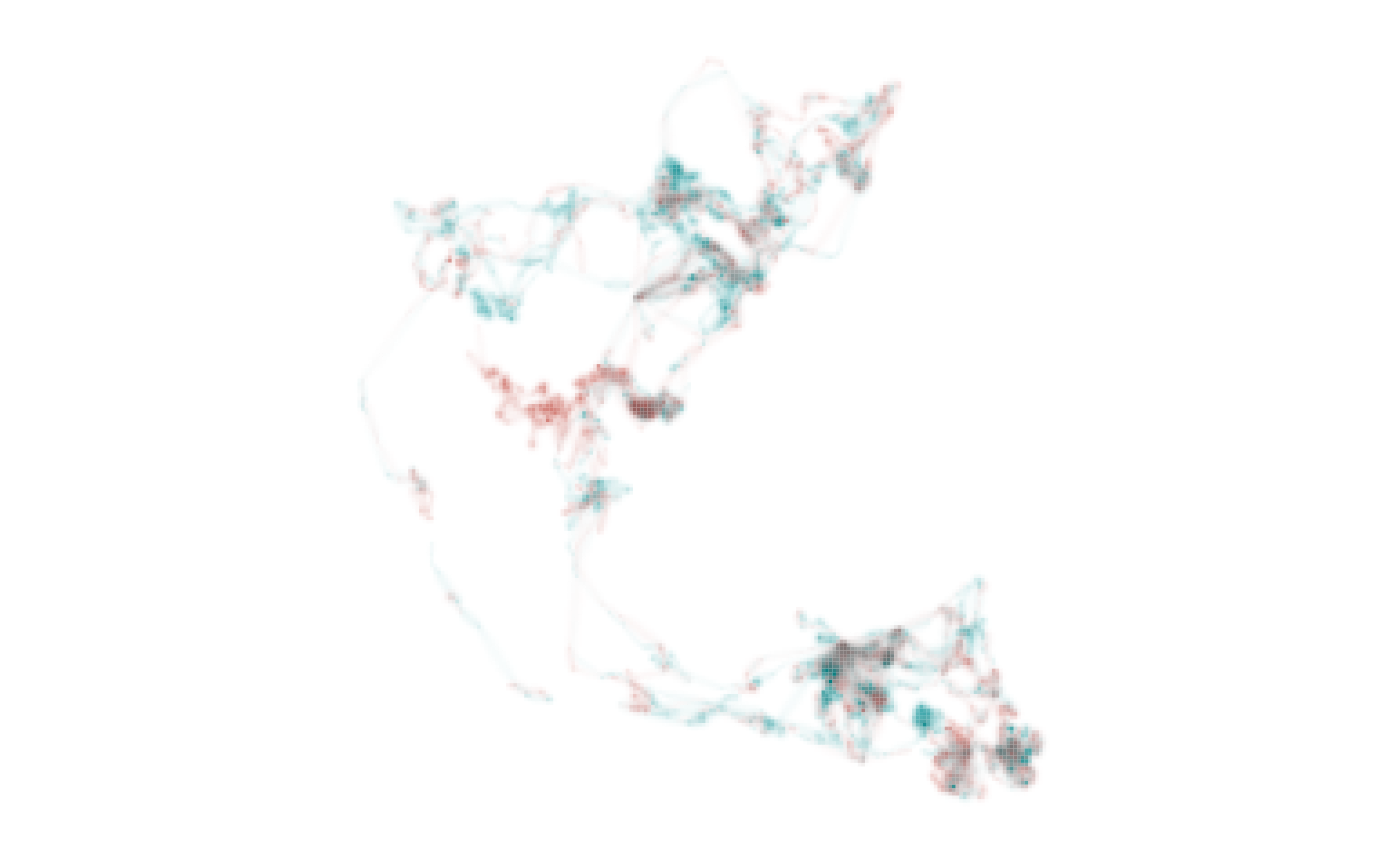# return RasterStack containing RGBa values
m <- map_single(r, pal, lambda_i = -5, return_type = "stack")

# visualize RGBa values
library(raster)
#> Loading required package: sp
plotRGB(m, 1, 2, 3, alpha = as.vector(m[[4]]))